Intern Spotlight: Samuel Chen

MIT FCU was so excited to host three interns throughout the month of January as part of the MIT PKG internship program. This year's theme was Tech for Social Good, and one of our marketing interns, Samuel Chen, broke down how to create a personal budget using Excel.

How to Create a Personal Budget Using Excel

Budgeting and investing are crucial foundational pillars for long-term financial health and independence. For many, college is the first opportunity for young adults to manage their personal finances. By learning to budget, students can efficiently allocate funds for essential expenses such as tuition, housing, and transportation while managing excess spending. These financial decisions are vital in managing student debt, a common challenge among college attendees. Moreover, even in small amounts, investing plays a critical role in a student's financial growth. Early investments harness the power of compound interest, paving the way for substantial long-term gains, which are instrumental in achieving financial goals like retirement savings. These practices help students in immediate financial management and instill lifelong habits essential to building stability and independence post-graduation. Budgeting and investing are not just about navigating the present; they are critical tools in shaping your financial future.

In this article, I will go through the steps to help individuals automate their finances in Excel. These steps are intended to be personalized to the reader's financial experiences. The two main sections of the article are the personal budget and investment simulator. 

Section 1: Personal Budget

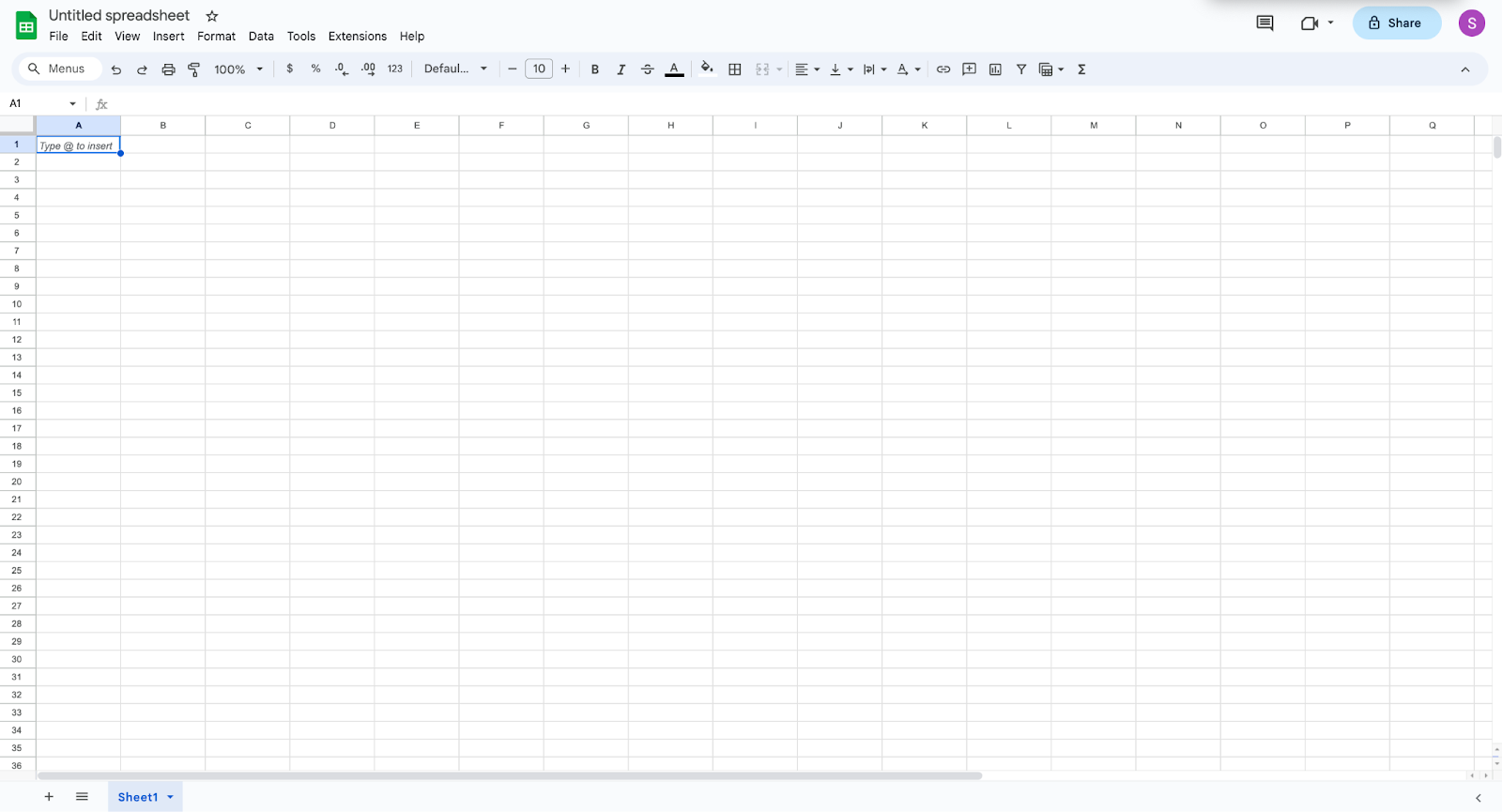
1. Start by creating a blank spreadsheet.

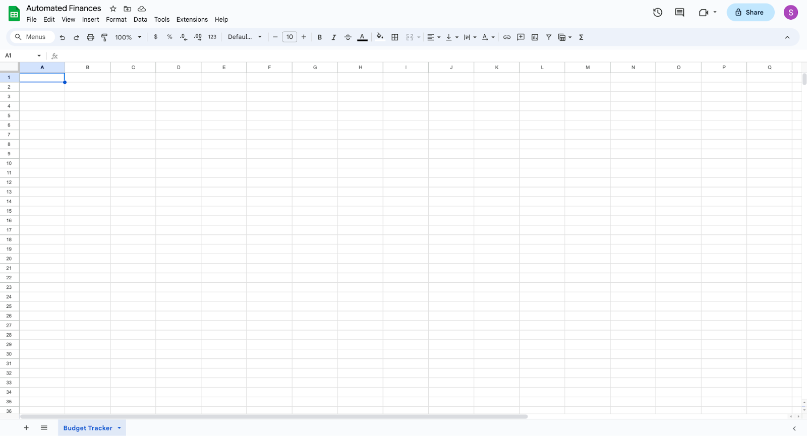
2. Rename your file “Automated Finances” in the top left corner and rename the specific sheet “Budget Tracker” in the bottom left corner.

3. Create major categories to break down your spending into several areas. Leave space between the categories for subcategories. I chose home, transportation, education, leisure, and medical, but you should create categories that match your spending habits. At the bottom of the sheet, make a total line for the sum of the expenses.

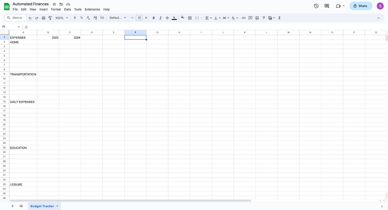
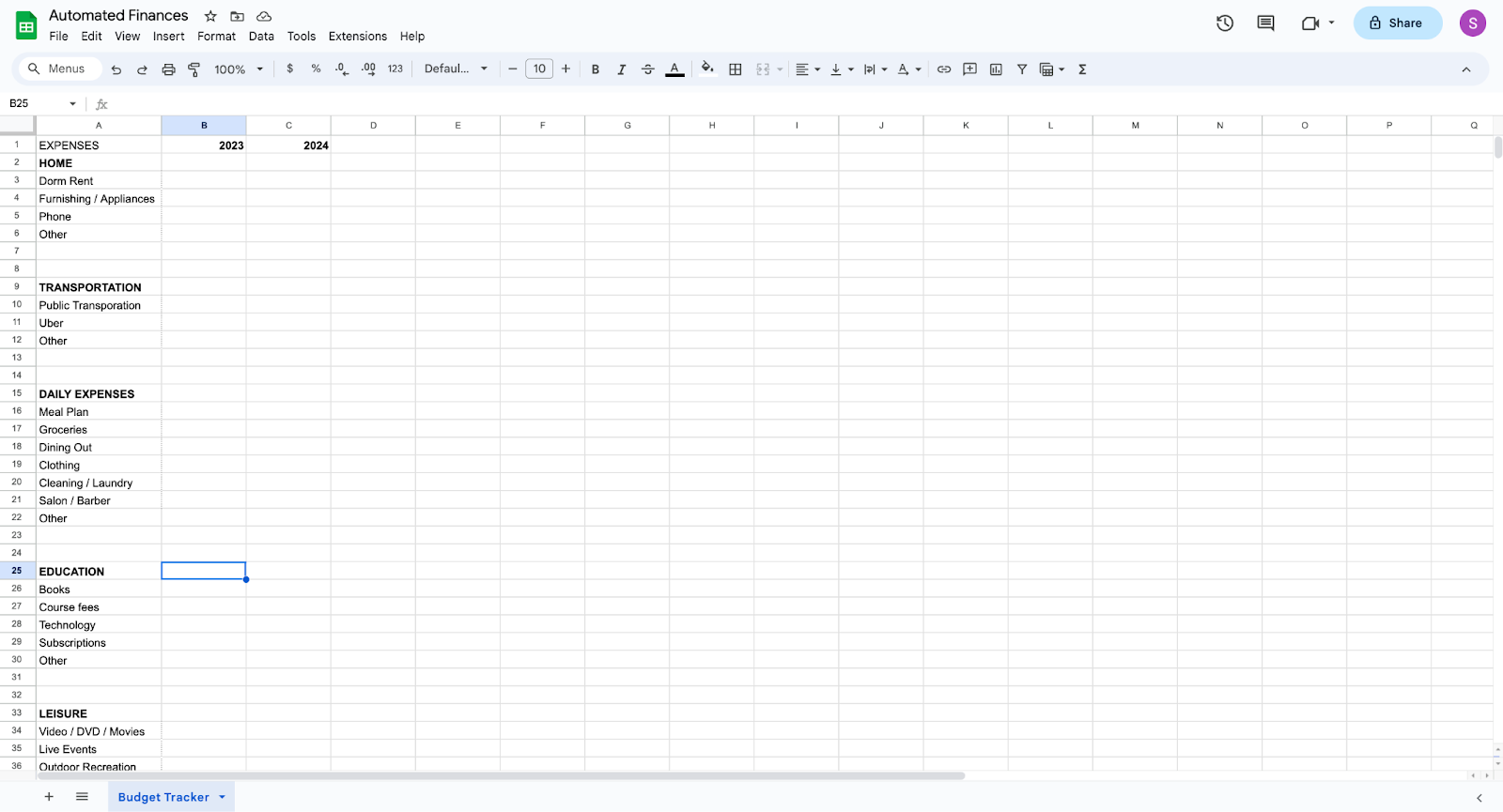
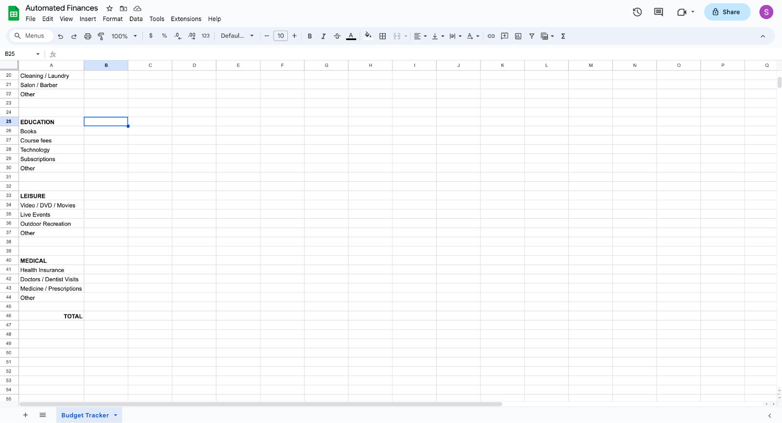
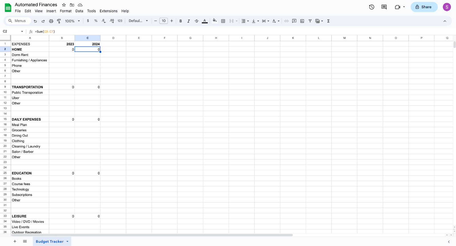
4. Create subcategories of expenses under the titles you created in step 3. I wrote down three to six subcategories for each title. It is important to differentiate which subcategories are necessary and unnecessary expenses. In my example, the subcategories under home, transportation, daily expenses, education, and medical are essential expenses. The subcategories under leisure are optional expenses.

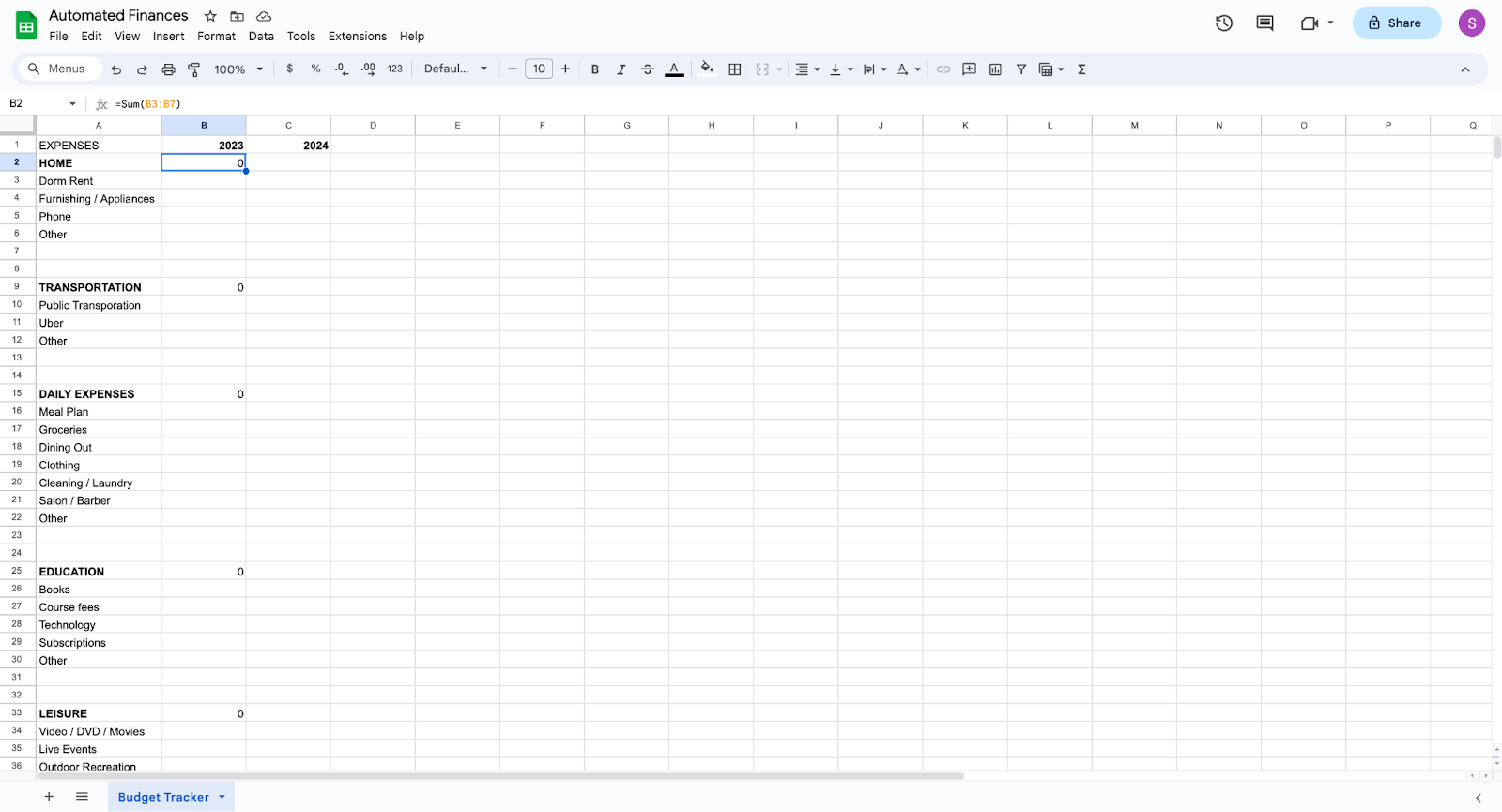
5. In the cell to the right of the major category titles, type the equation =Sum(Cell1 : Cell2). Cell 1 represents the highest cell, and cell 2 denotes the lowest cell contained by the major category. This sum will add all the expenses of the subcategories. Typically, college students spend the most on food and home-related expenses, but it is important to see your expense breakdown. 

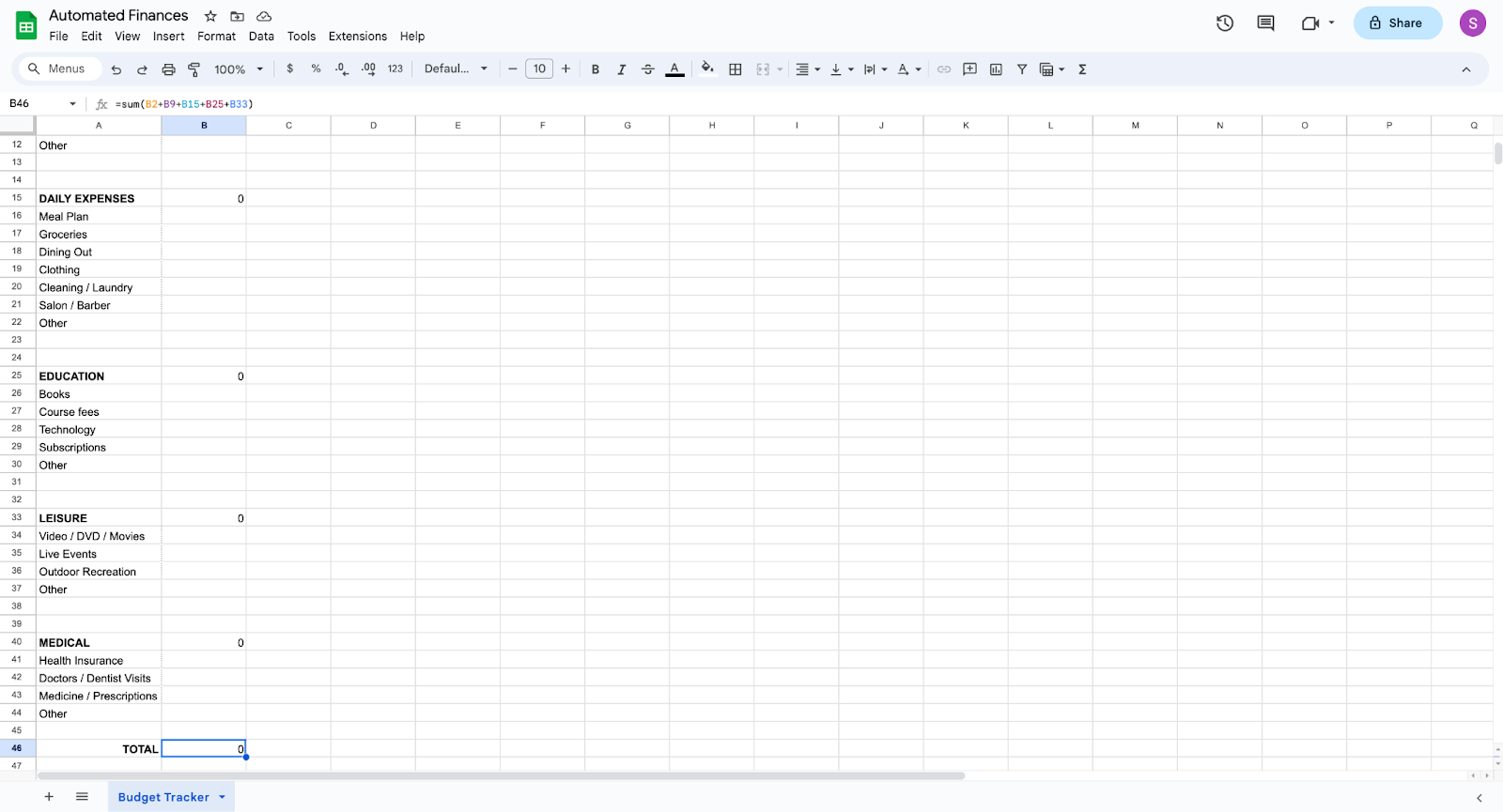
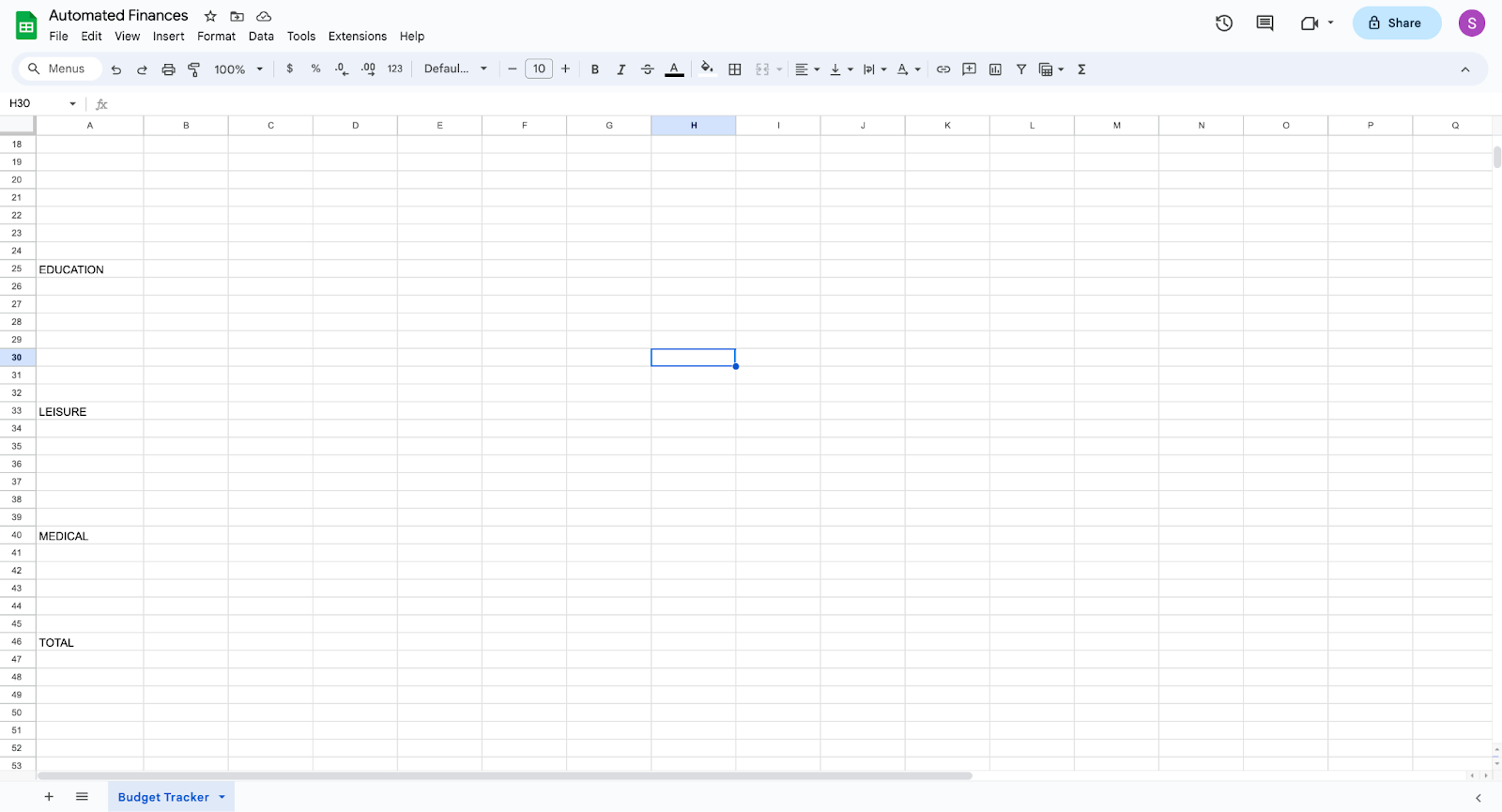
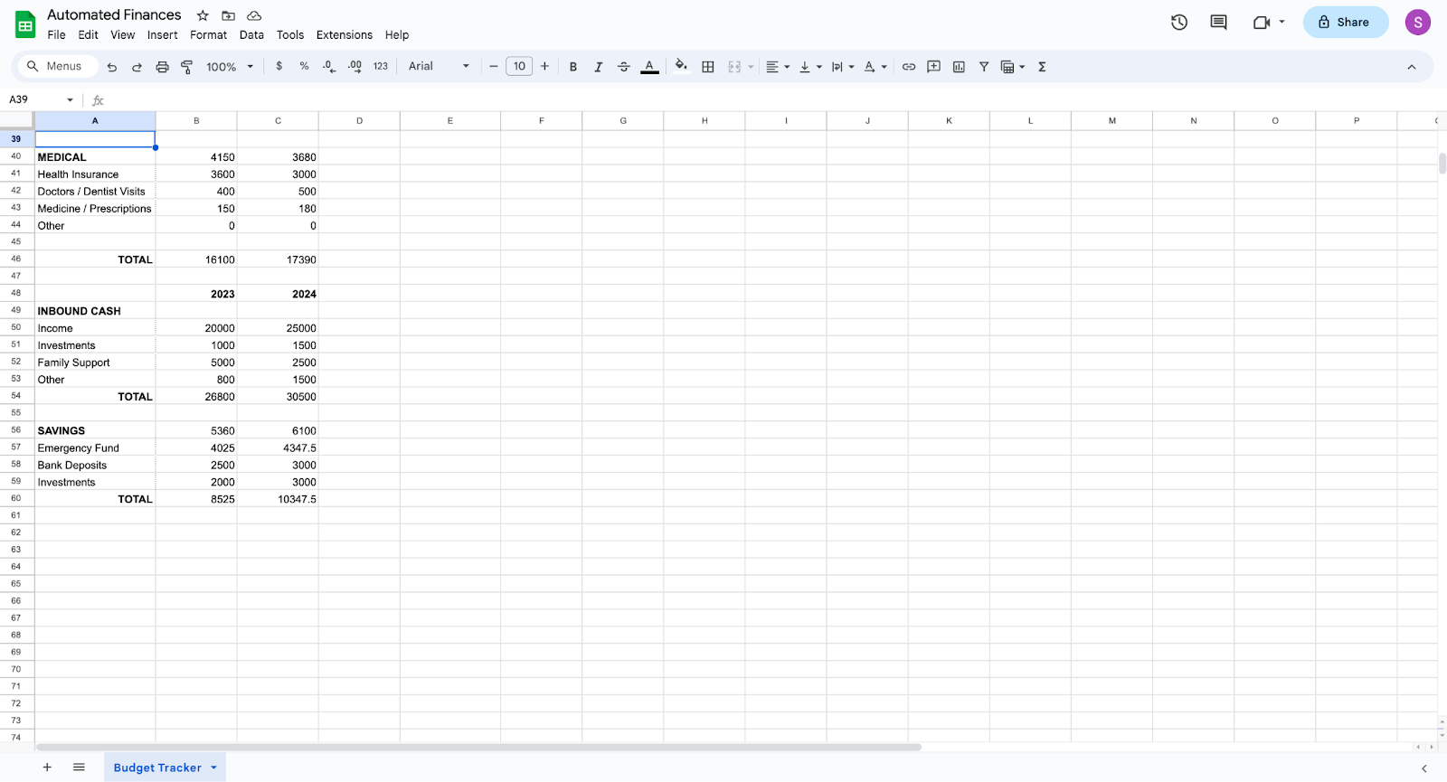
6. Under total, use the equation =Sum(Total Expense Cell 1 + Total Expense Cell 2 + Total Expense Cell 3…)  This will calculate your total expenses for the year. MIT projects students to spend around $23,000 annually, but it fluctuates depending on student situations.

7. Copy all the cells with equations from Column B and paste it into Column C. The equations will automatically update to represent Column C. This creates a column with the projection budget for 2024. A projection budget is crucial because it acts as a financial blueprint and ensures the efficient allocation of funds. 

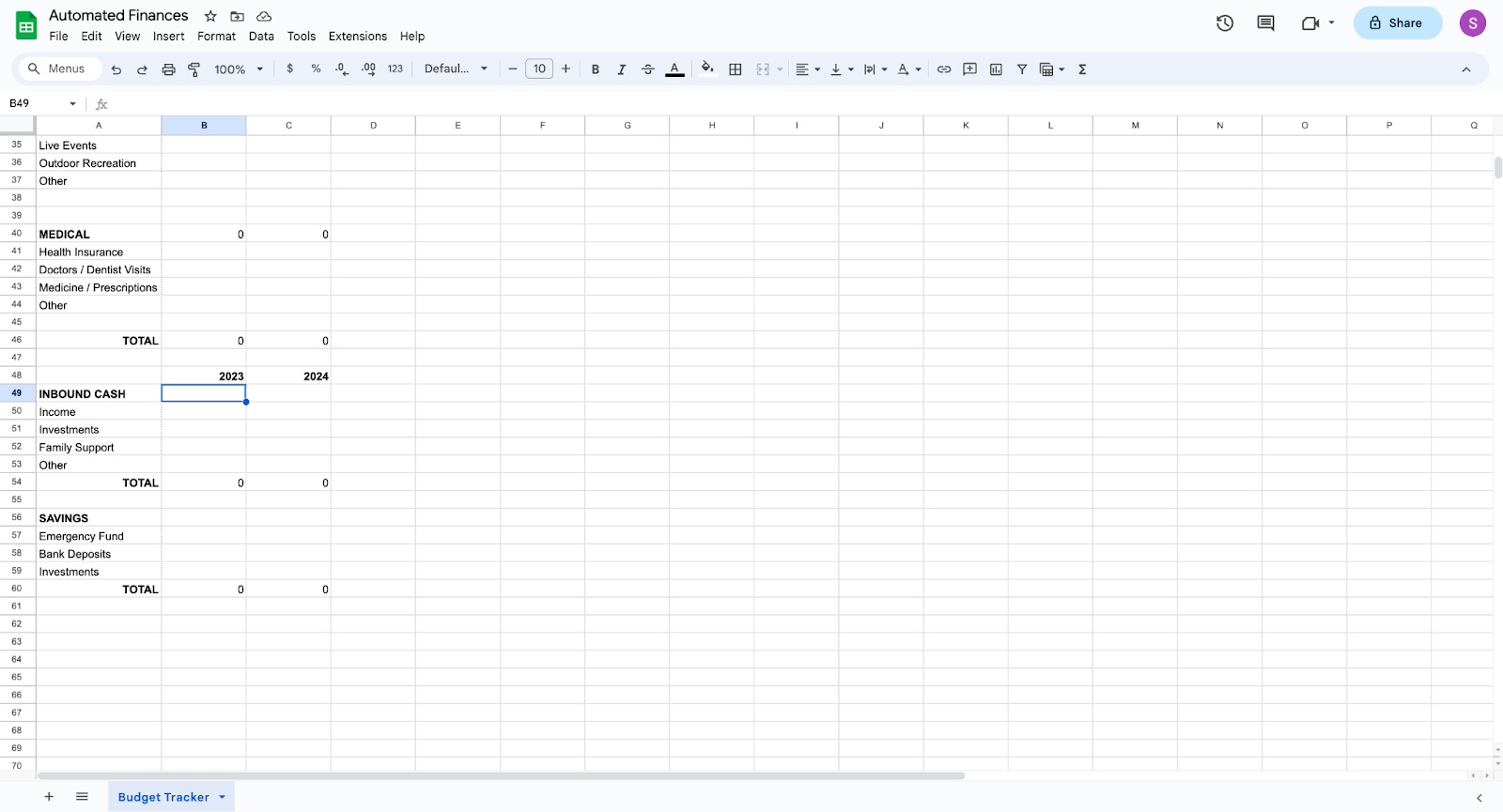
8. Underneath the expenses, create two major categories. Inbound Cash and Savings. Create subcategories under inbound cash and savings. I used income, investments, and family support as sources of inbound cash and emergency funds, bank deposits, and investments as saving avenues.

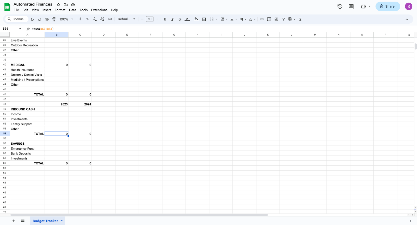
9. Use the sum equation =Sum(Cell 1: Cell 2) to add the cells from each subcategory under Inbound Cash and Savings. Copy the equations from your 2023 budget to the 2024 budget column. These calculations will deliver the totals for inbound cash and savings. Tracking your incoming cash and savings is essential to evaluate your financial goals, provide insight into income patterns, and make informed financial decisions in the future.

10. At the top of the savings category, create a goal for the percentage of your inbound cash you would like to save. Use the equation =Cell 1 * X. Cell 1 represents the total inbound cash cell, and X denotes the percentage of income in decimal form. I chose 0.2 because financial experts recommend saving 20% of your income. However, it will vary based on students' working hours, expenses, and family support.

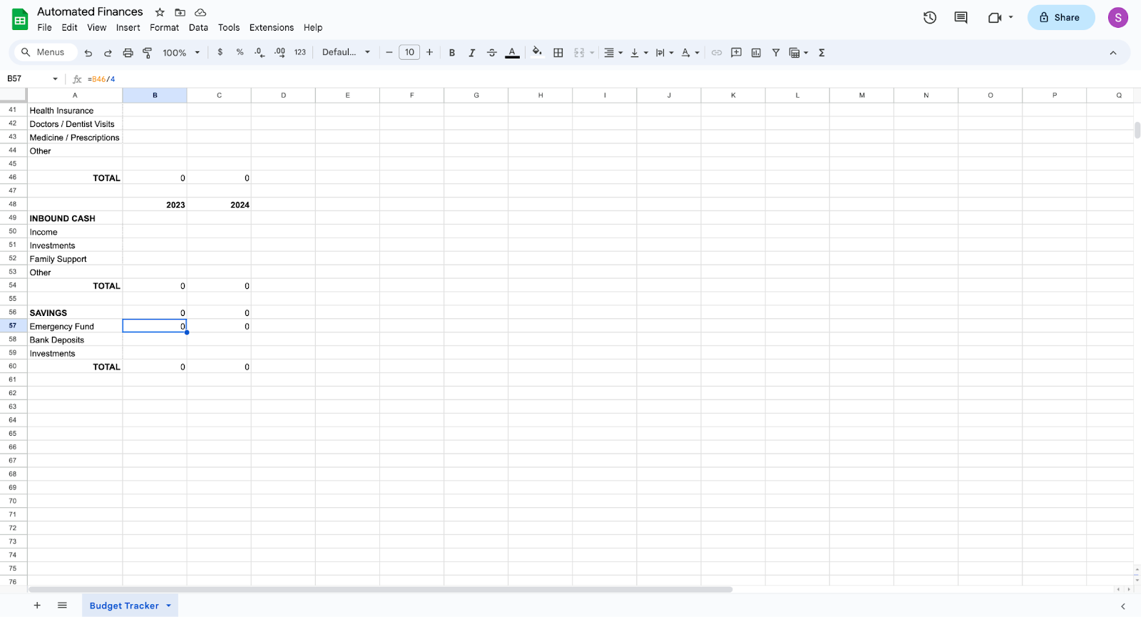
11. In the emergency fund row, I used the equation =Total Spending Cell / 4. This is calculated based on financial experts' recommendations of three months of emergency fund savings. However, it is common for students to have lower emergency funds due to access to financial help from parents or guardians.

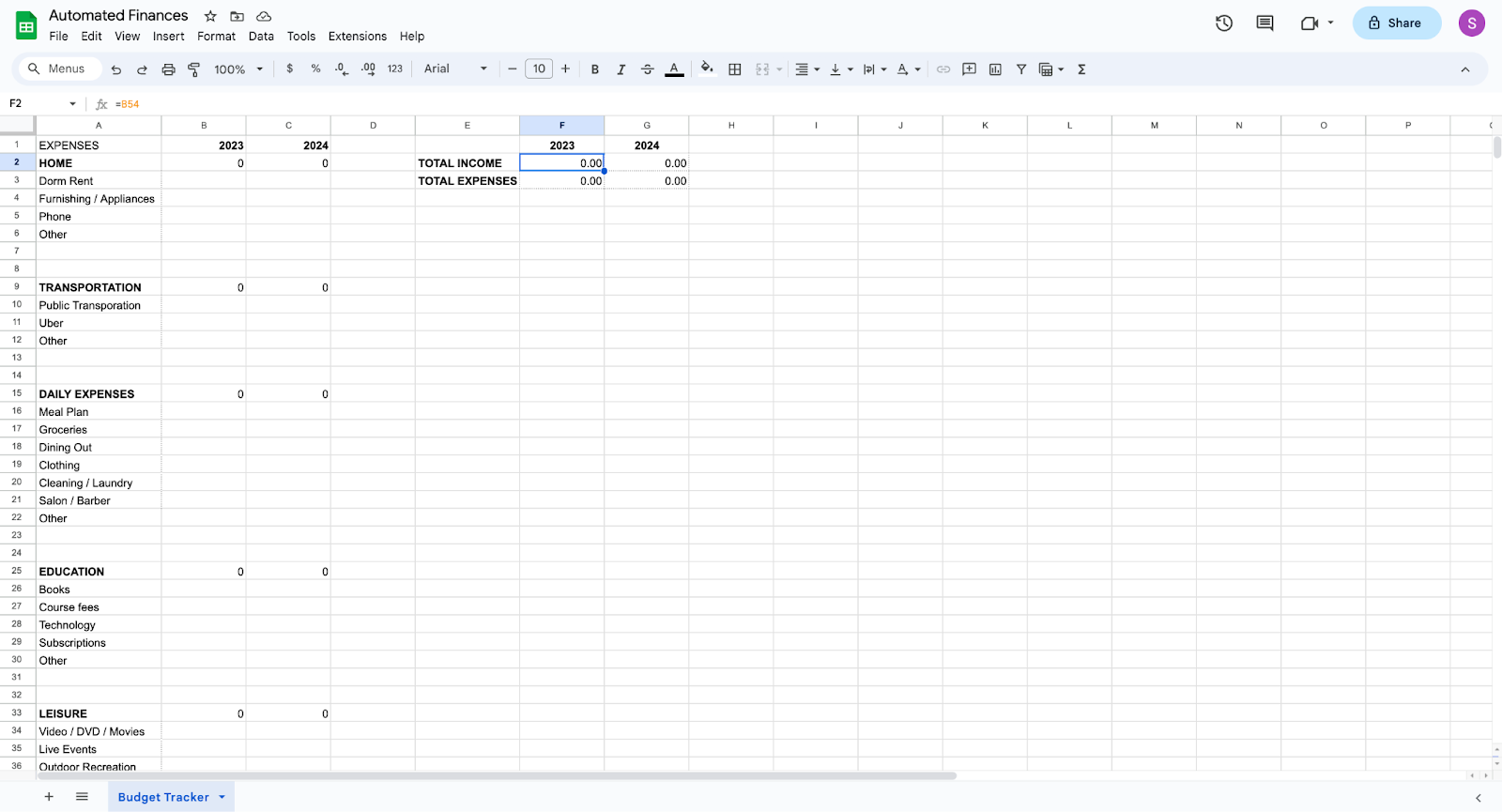
12. To make the spreadsheet easier to read, I created total income and total expenses lines near the top of the sheet on the right side. Use the equation =Total Income Cell and =Total Expenses Cell that were calculated at the bottom of the sheet.

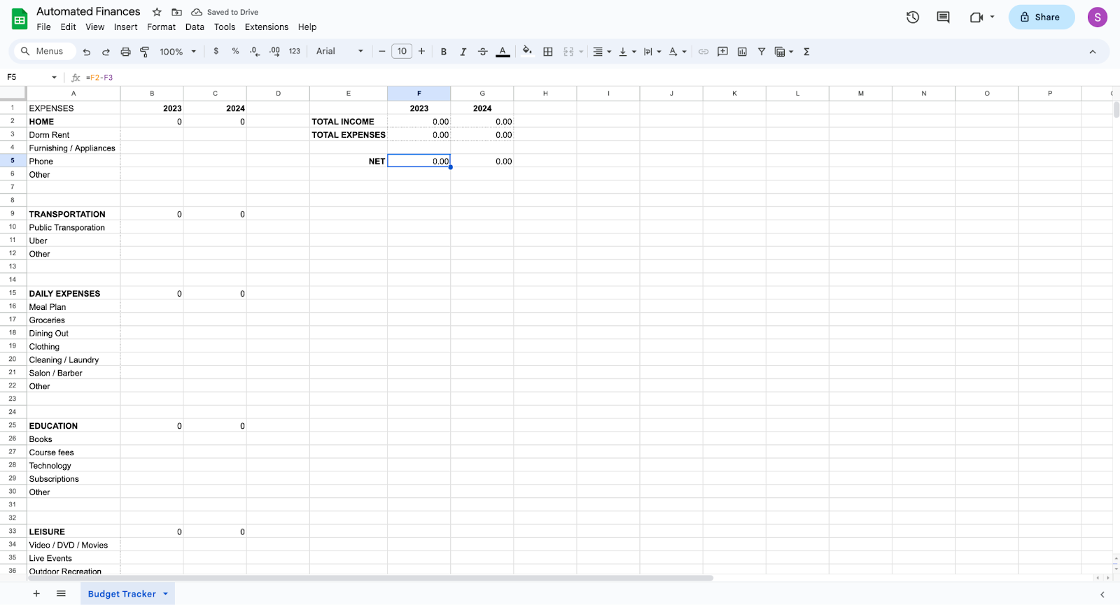
13. Create a net income line and use the equation =Total Income - Total Expenses. This will calculate the excess money you can save or have on hand. 

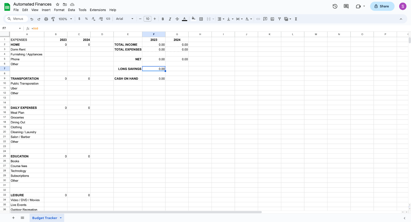
14. Create Long Savings and Cash on Hand lines to get a better understanding of your budget. For Long Savings, use the equation = Savings Cell at the bottom of the sheet. For Cash on Hand, use the equation  = Net Income Cell - Long Savings Cell. For college students, any contributions to long-term savings are impressive and will pay large dividends in the future. Across the country, less than one-third of college students have more than $1000 saved.

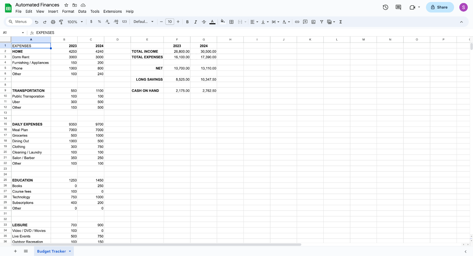
15. Begin inserting values under each subcategory of expenses. Check that the equations for total spending are correct.

Section 2: Investment Simulator

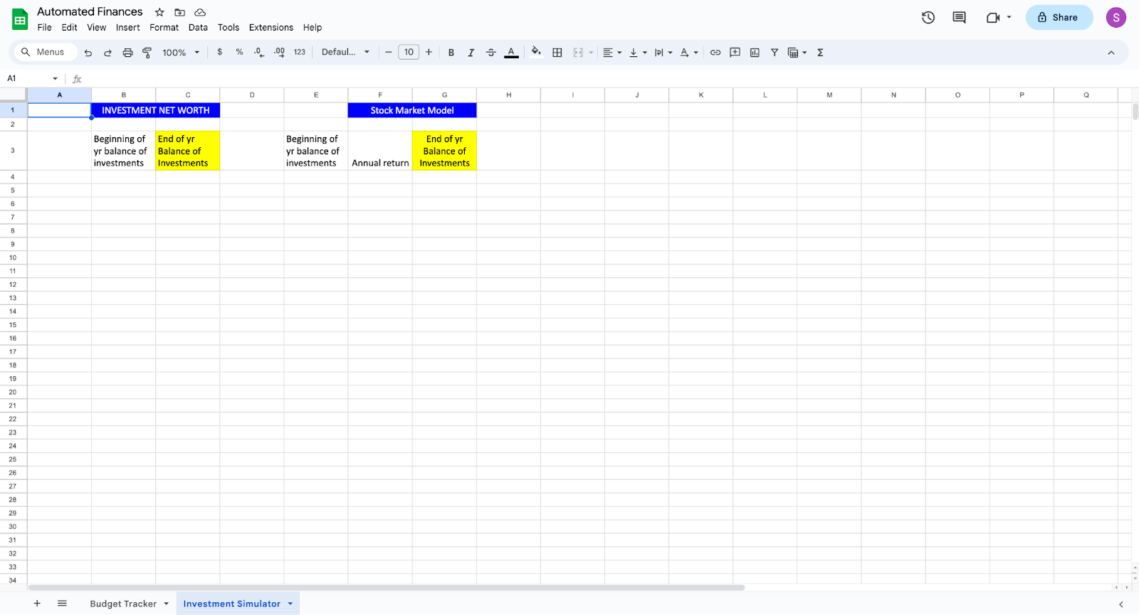
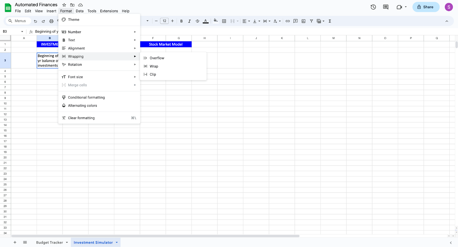
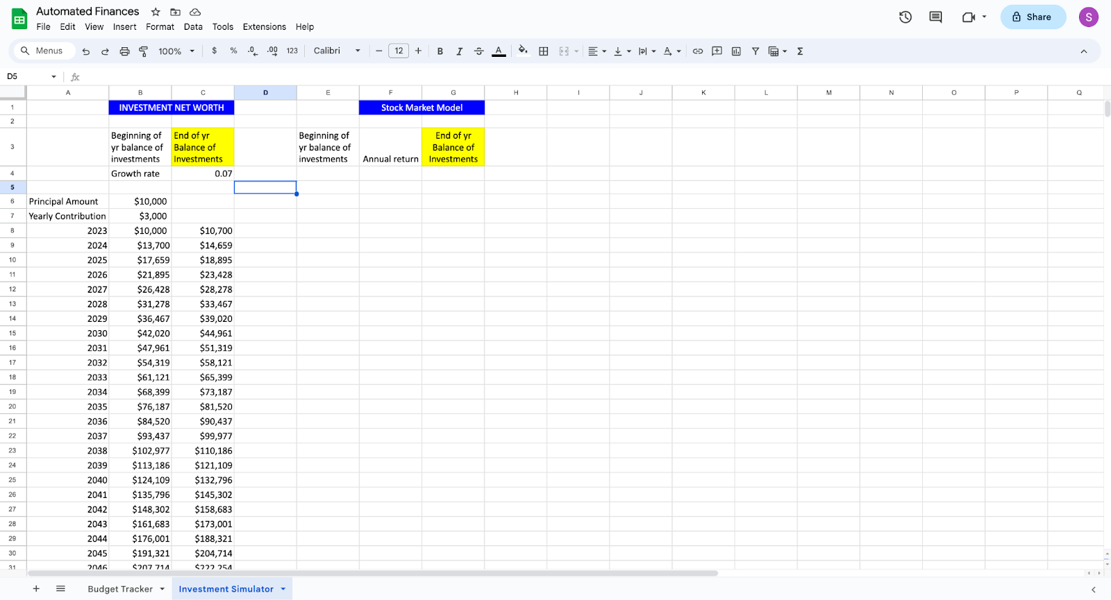
1. Start by creating the headings shown in the example photo above. To wrap text, go to format, wrapping, and wrap.

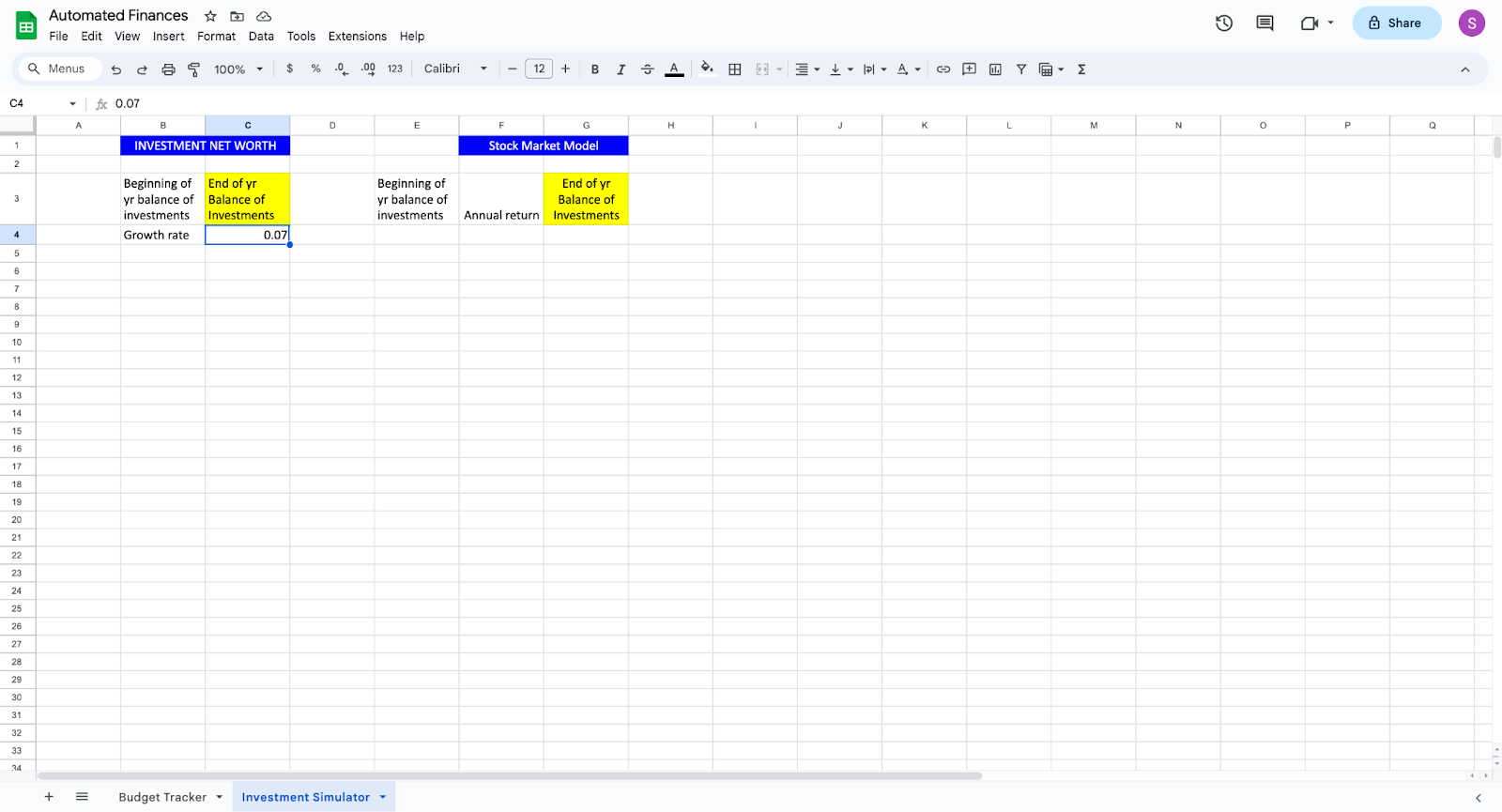
2. Create a growth rate cell and set any decimal growth rate. I chose 7% because the stock market has grown an average of 7% for the past 50 years when adjusted for inflation. You can use a more conservative or aggressive growth rate. I often use a more conservative growth rate for a safe financial projection.

3. Create a principal amount and yearly contribution cell. The principal amount should be set to your current savings in your investment fund. The yearly contribution should be calculated based on your budget tracker slide. A recommended investment contribution is 10% of your annual income, but that can be a challenging goal for college students.

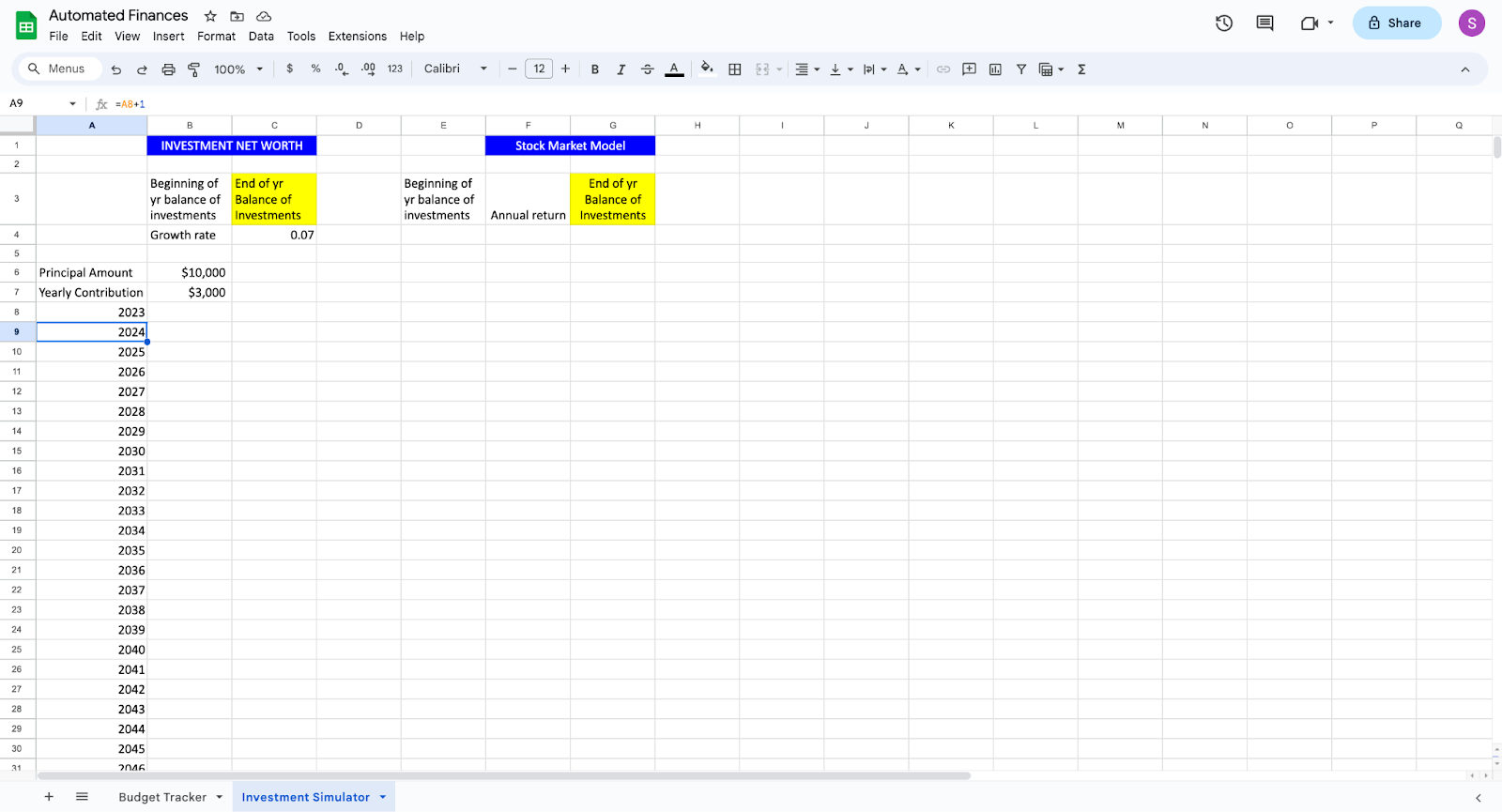
4. Form a column of year values on the furthest left column. To simplify the process, use the equation =Cell above + 1. You can write the formula in one cell and copy and paste it for the following 50 cells.

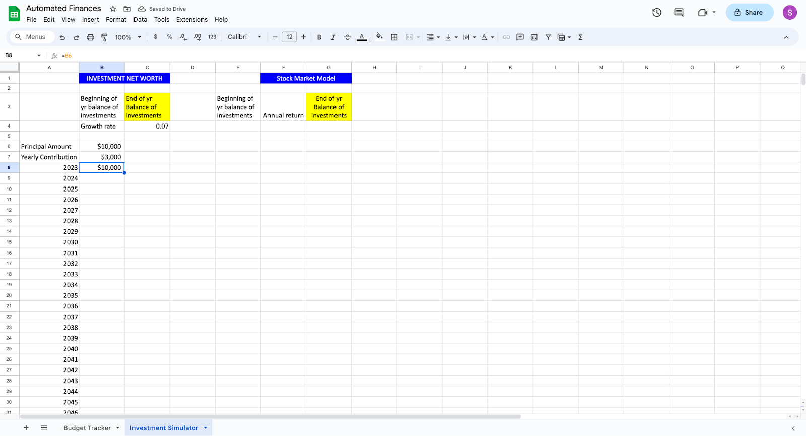
5. Set the first beginning of year balance to the principal amount.

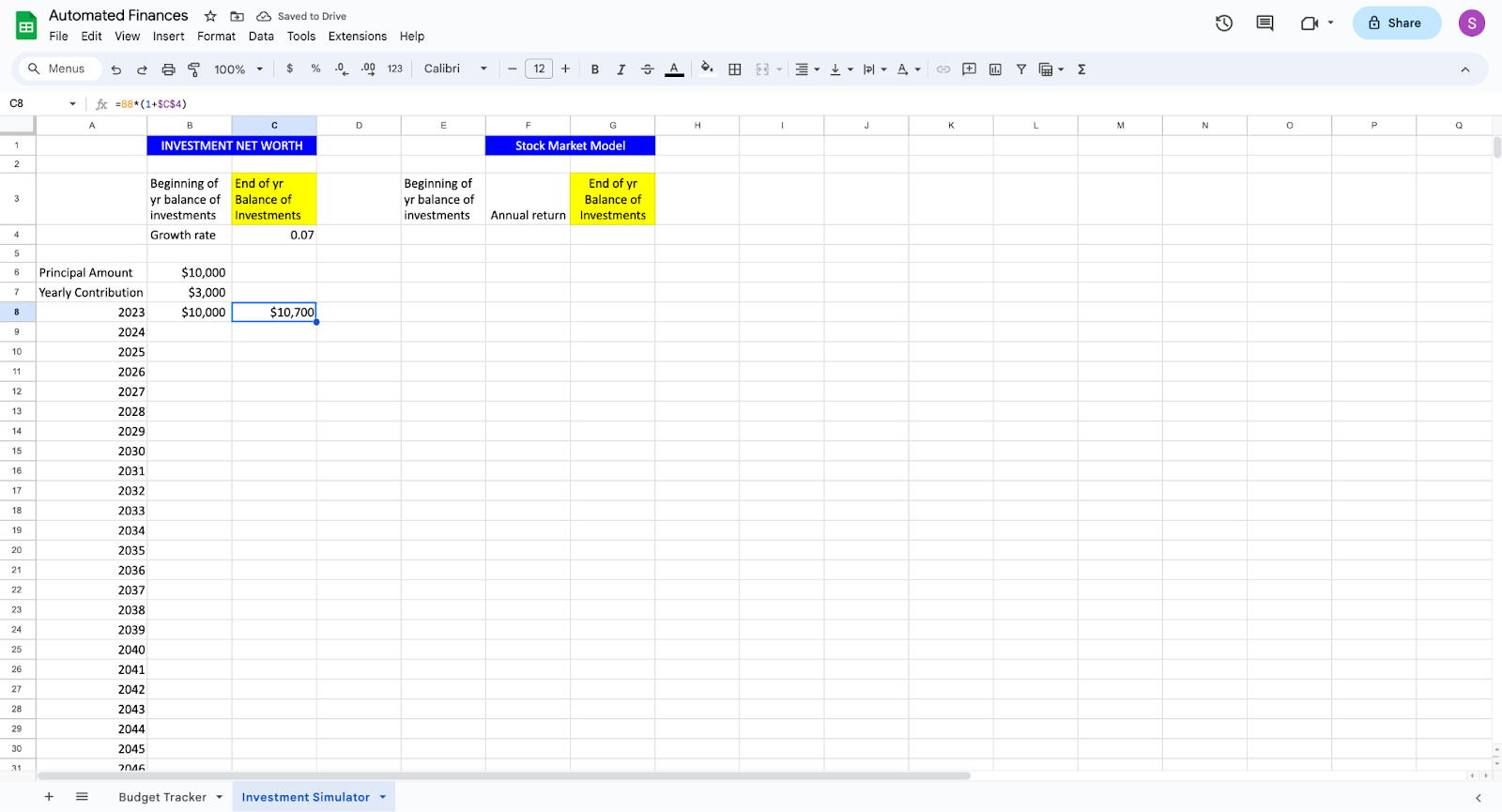
6. Use the equation =Beginning of Year Cell * (1+Growth Rate Cell) to calculate the end-of-year investment value. You must use dollar signs in front of the column and row of the cell. This ensures the cell reference will not change when the equation is copied and pasted to other cells. This equation calculates the growth of your investment account in that year. While the year-to-year growth may appear minimal, the power of compounding investments leads to an impressive final total. 

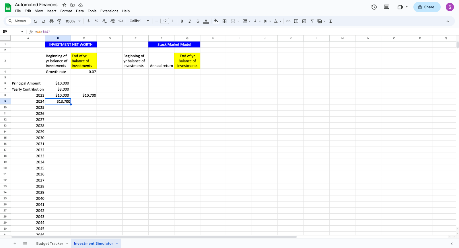
7. To calculate the following year’s starting investment value, we will use the previous year's balance and add the yearly contribution. The equation will be =End of yr Balance Cell + Yearly Contribution Cell. For this equation, we must use dollar signs before the column and row of the yearly contribution cell notation. 

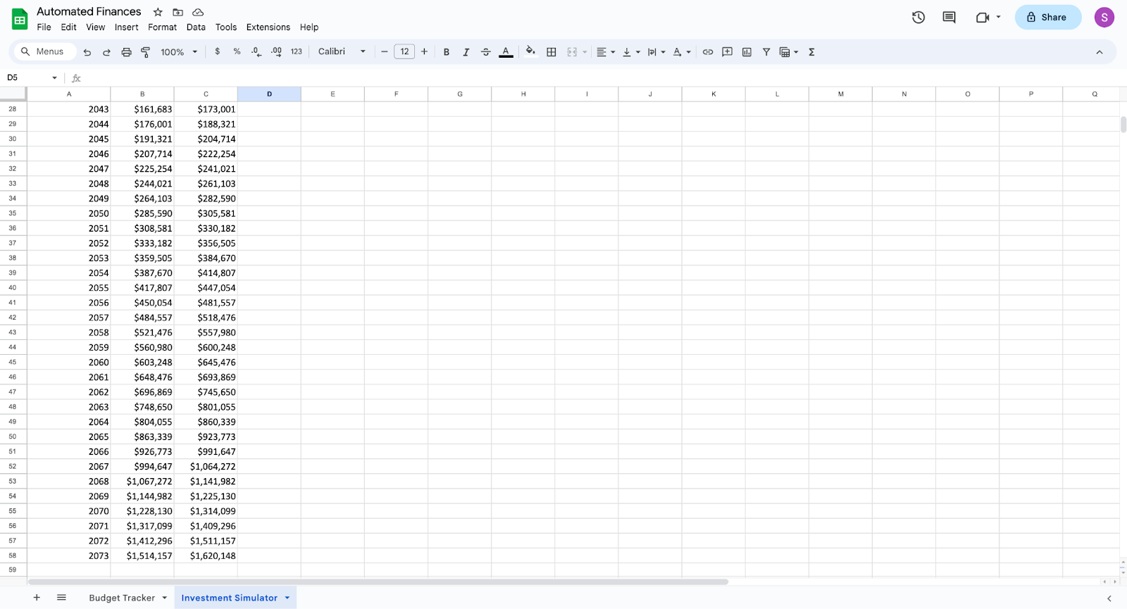
9. Copy and paste the equation down the columns. You must paste the equations down their columns and not across columns.

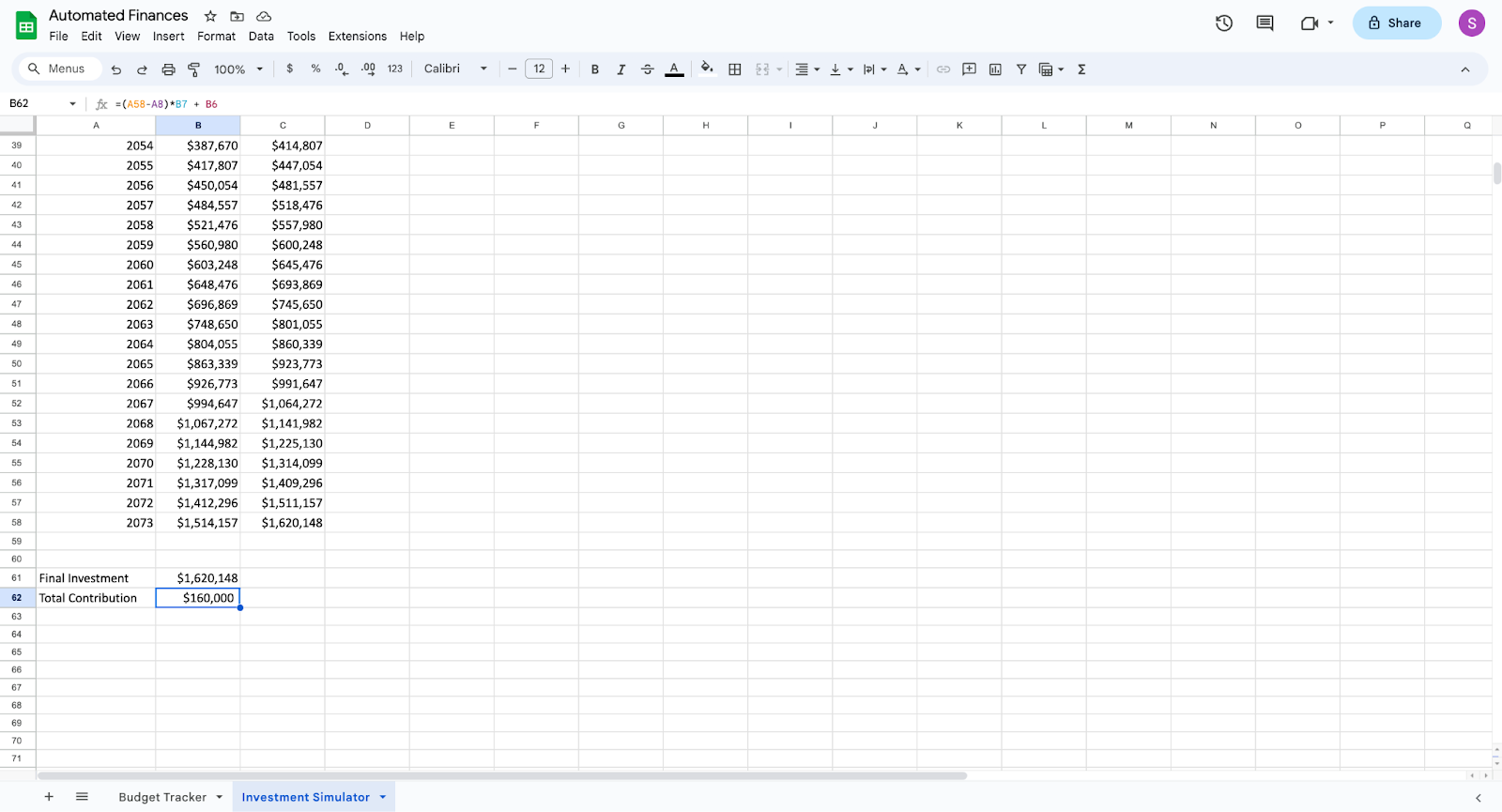
10. Create a final investment value row and assign it to equal the cell with the final investment balance. Create a total contribution cell using the equation =(Last Year Cell - First Year Cell) * Yearly Contribution Cell + Principal Amount. This equation should look similar to this: (2073-2023) * $3,000 + $10,000. The equation will calculate the amount of money you contributed to the investment account over the years. In my example above, I contributed $160,000 but ended with $1,620,148 through compounding investments. 

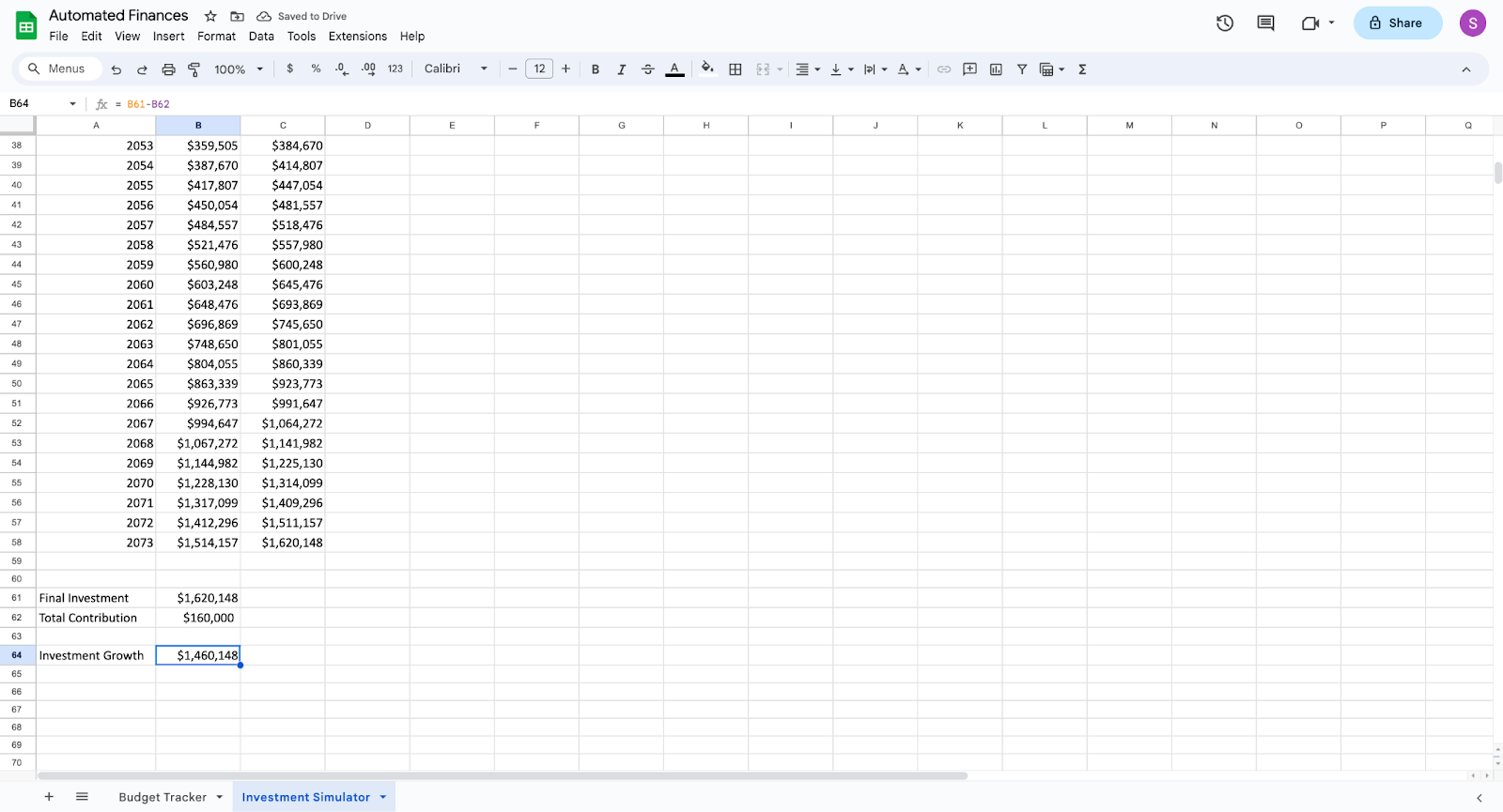
11. Create an investment growth row by using the equation =Total Investment Cell - Total Contribution Cell. This calculates the pure investment growth by removing the amount you contributed. The investment growth of over 1 million dollars shows the power of time for investments.

This investment simulator was built to show how investments help your savings grow and outpace inflation over time, build wealth for long-term financial goals like retirement, and provide additional income streams.